Introduction
List of abbreviations
Pointillist graphing
OpenGL live demos
Background
Why OpenGL in 2016?
Examples / tutorials
Modern vs. legacy OpenGL
Limited canvas size and resolution
Linear IFS
Nonlinear functions: fragment shaders and inverses
Parameter evolution
Stages overlay
Camera loop / continuous iteration
Alpha, transparency and blend
Colour manipulation and creation / non-iterated demos
Initial sets / image sources
Hardware and performance notes
Vertex shaders: pointillist graphing with forward functions in OpenGL
Problems and solutions
3D functions and iterations
Geometry shaders
Ray tracing
Shading/lighting vs. fractals
What follows are informal and incomplete notes on how I make my art. This is a work in progress started on 2018-07-18.
| ETG | escape-time graph |
| FB | framebuffer |
| IFS | iterated function system |
I began making art with iterated function systems in June 2015. I was taking the course "Johdatus fraktaaligeometriaan" (Introduction to fractal geometry) by Antti Käenmäki at the University of Jyväskylä. One night I decided to write a script to check some of my work visually, and things grew from there. My approach is outlined in my Bridges 2016 paper (Colour version).
I continue to use and develop that method, with the calculations done in Julia and the results presented in gnuplot. These are tied together with Bash scripts, whose importance is not to be underestimated. For example, to render animations, these scripts distribute the work to different CPUs on different machines.
I started hacking together my live demo system in March 2016, as I was preparing my first live show for Yläkaupungin yö. I already had scripts where the Julia-gnuplot approach generated new pictures with random parameters every few seconds for a slide show, and a number of pre-made animations. I had realized there were I/O bottlenecks with my setup, so the next version would have to work within a GPU.
OpenGL was not the obvious starting point, given the more flexible and powerful approaches that had already been around for a few years: OpenCL and CUDA (though these would generally use OpenGL to present the picture). The new unified framework Vulkan was also getting into mainstream.
However, my primary workstation/laptop did not even have OpenCL. While I did have newer/stronger machines around, I was already envisioning exhibitions with multiple small/cheap machines, so I wanted to keep the hardware requirements low. There was also a ton of literature, tutorials and examples on OpenGL, and I knew it could do fairly complex (pun intended) and flexible computations via shaders. (In fact, people were using OpenGL for non-graphics computing in the very early 2000s. These ideas were eventually formalized and developed into CUDA and OpenCL.)
Using Python's PyOpenGL was obvious early on, as I didn't need much power on the CPU side, and I knew Python well. Julia didn't have a complete OpenGL wrapper at the time, while Python has many other useful libraries I would need later, such as Numpy.
The choice of OpenGL had a number of effects on my art, as I moved from the math of abstract points into an image-manipulation approach. There were a lot of new limitations and quirks, which often turned out to make interesting results.
Iterating shader passes on an image needs render to texture, and Leovt's example turned out a good starting point. Pyglet also turned out better than Pygame for my purposes; both provide windowing and keyboard controls among other things.
Another important example was glslmandelbrot by Jonas Wagner. It produces the familiar Mandelbrot set images using the Escape-time algorithm (alternative link), and I call the resulting graphs ETG for short. This was not directly relevant to my art, but this was a good starting point for using and controlling shaders. In fact, I soon extended this into my own general ETG system, and integrated it with my IFS scripts (early example).
A lot of the examples/tutorials found online are still using Legacy OpenGL, i.e. pre-3.0 or pre-2008. This can include fairly recent ones, presumably because the author learned OpenGL in the olden days. Functions such as glColor, glVertex, glMatrixMode, glRotatef are tell-tales of the old fixed-function model. The code will usually run on regular computers due to compatibility layers, but for learning purposes it should be avoided. Of course, the examples may still have useful ideas, but the code itself should be updated.
Modern OpenGL may seem more involved because tools such as projection matrices are not ready-made. One reason for this is to make the GPU a more general processor, and projections of 3D scenes are just one of the ways you can use it. I like putting all the GPU power into my 2D works, without any unused 3D engines hanging about. If you want 3D you need to write some code.
The "canvas" in OpenGL is defined by coordinates of either [0, 1]2 (texture lookup) or [-1, 1]2 (target position). I usually scale these in my shaders so as to do math in [-2, 2]2 or [-10, 10]2 or something. In any case, they must be fixed at some point, and there is no simple way to auto-scale these depending on the image. The point of live demos is usually having randomly varying parameters, and you need extra room for that, but not too much as that would leave things small with huge margins.
Resolution becomes crucial in iterated OpenGL, because initial fine points will generally end up more or less blurred. Things must be quantized into the MxN grid at every iteration, and this often means interpolation blur. (Though the nearest-point approach can sometimes make neat retro/glitch effects.) For higher quality, I sometimes use FBs larger than the final screen.
In contrast, the mathematical points in my Julia-gnuplot approach have practically unlimited range and resolution, and gnuplot can auto-scale its output to fit the image nicely. But even then I often use larger-than-needed plotting resolutions to smooth things out, and I sometimes need to set my own ranges. (In any math problem, one should generally keep high precision and only round at the end.)
Linear functions can be realized in basic OpenGL methods without shader math. In fact, this is how I started — by noting that a linear function means taking a photo and moving it around. Then you can take a photo of the result and you have iteration.
Such linear mappings are defined by vertex placement. (Technically, these can be somewhat nonlinear, in case the target shape is not a square/rectangle/parallelogram, depending on your definition of linearity.) For starters, identity mapping:
These are the corresponding texture and target coordinates of the SW, SE, NE and NW corners in this order (recall the above canvas limits). The following mapping would rotate by -pi/4 and multiply by 1/sqrt(2) while keeping it centred:(0, 0) -> (-1, -1) (1, 0) -> (1, -1) (1, 1) -> (1, 1) (0, 1) -> (-1, 1)
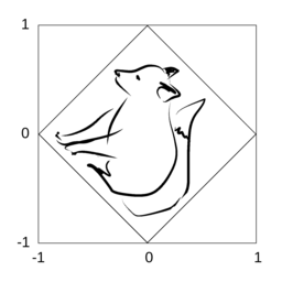
In other words, I take the corners of the texture, and place them somewhere on the target FB (generally within corners, anything outside will be cut out). This example is illustrated in the picture, fox art courtesy of Aino Martiskainen.(0, 0) -> (-1, 0) (1, 0) -> (0, -1) (1, 1) -> (1, 0) (0, 1) -> (0, 1)
The basic photo-collage operations of rotation and translation, etc., cannot capture nonlinear transformations. Likewise, vertex positioning would fail to reproduce such mappings. The solution is found in shader programs, but there is a slight complication: the functions must be defined in the inverse direction.
Modern OpenGL uses shader programs all the time, but for linear mappings they are simple pass-through boilerplate. For each output pixel, the fragment shader decides the colour, often by looking up an input pixel whose position depends on the output position. For graphics processing it is a sensible direction: you only calculate what you'll see.
This stage provides a kind of workaround for the limited canvas size: if your lookup position is beyond 0 or 1, you can wrap it around (mod 1 or a mirroring version). This can be done with OpenGL settings, no need to change your shader code. It can make interestingly repeating, non-periodic patterns. (For wraparound in a linear IFS, write the linear function in a shader.)
Inverting functions is not always feasible. In some cases this makes things easier, for instance with Julia sets as they can keep the same form as they do in ETG. In other cases you get nice surprises as you try familiar functions in the inverse way.
At best, you will learn to think about functions in this lookup direction more naturally and take advantage of it. Mathematicians will find themselves right at home; preimages of sets are at the heart of topology and measure theory, for example.
I now have unified the linear and nonlinear approaches, since often a function can have a linear outer function, and this makes it easier on the GPU.
As a simple example, the Julia-set polynomial z2 + c has two parameters: Re(c) and Im(c). The parameter space is a 2D plane. In practice, one would use a box just around the Mandelbrot set to get nice Julia sets. (This video shows one such path along with its Julias, albeit not very box-like.)
The total n parameters of all functions can be regarded as a point in an n-dimensional box. To make my demos alive, I fly this point around the box using a kind of random walk. This post on my Facebook page elaborates a little, with another video.
One key idea in my Bridges 2016 paper was overlaying the stages of iteration into a single graph, so that was an important aim with OpenGL too. It was relatively straightforward, once every iteration was given its own FB. The pictures are white on transparent during iterations, and they are coloured by multiplication upon the overlay stage.
This method is relatively heavy due to the number of iterations per displayed frame. First, there are the individual iterations, typically 10. In addition, the overlay step involves one rendering per visible stage, so there are often 15...20 renders per frame, or about 1000 renders/sec with typical framerates.
An alternative method draws from real-life video loops, which are nice to play with if you have a video camera connected to a display. In IFS parlance, it would be a single linear function, so not particularly interesting. Adding multiple displays that show the same feed makes a proper IFS. The camera needs to see all of them at least to some extent; the background visible outside/between the displays will provide the light that circulates through the system.
In my IFS setup, this just means rendering the iterated images back onto the original. I use a cyclical buffer of several FBs to simulate/exaggerate the physical delay. As in the real setup, this becomes interesting as the functions themselves change during the iterations. Sometimes I leave out the delay buffer to simulate a continuous flow process (example).
Performance-wise, the Camtinuum™ is particularly nice as there is only one iteration per frame. This is easily noticed on slower integrated GPUs, which would choke on the corresponding multi-stage demo.
To simulate proper IFS graphs, blend is essential. The images of each function must be overlaid so that the (transparent) background of one doesn't hide other images. Sometimes the usual "alpha blend" is not the best approach, and others may give interesting results. Blend-less hard overlay naturally simulates multi-display camera feedback (unless you have those transparent displays from SF movies). Max blend is good for simulating CRT afterglow, albeit that would be a separate single-function, single-stage postproc operation.
The gradient effect from my Bridges 2016 paper can be simulated by varying the alpha levels within functions, depending on their derivatives. It is often hard to get nice results so I use it quite sparingly (example with both Julia-gnuplot and OpenGL methods on similar functions).
In the stages overlay, alpha levels can be set separately for each iterate to get translucent colour mixing. This can be used as a rudimentary simulation of the pointillist effect, where the final iterates have higher point densities due to being smaller.
While we're doing image processing, functions can alter colour as well as position of pixels. This is a huge difference to the basic IFS math of colourless points. Frankly, I have not wandered very far in that direction; my colour processing endeavours have been limited to single-pass demos such as these two. Even this level has a lot to explore.
My Pointillist paper has a section on different initial sets, and that applies to OpenGL too. The basic initial sets are solid shapes instead of sets of separate points. Random pointsets can be simulated but they often end up blurry due to the usual quantization and interpolation. Thus I sometimes use large, blocky "points" for a kind of retro pixel look.
As noted above, pixels in OpenGL are not just points but they also carry colour, so full-colour images can be used as initial sets. These are best used with single or 2-3 iterations. Pyglet has simple ways to load image files into textures.
Live video input is the next level, and it makes a nice proof that these things do run in realtime. It is a little more involved: I use OpenCV with bit of GStreamer to read cameras and video files, then pygarrayimage for fast texture transfer.
Most of my demos run fairly smoothly on integrated Intel GPUs from early 2010s such as HD 3000, albeit in resolutions closer to VGA than Full HD. For serious work on serious resolutions, I've found that entry-level discrete GPUs such as Nvidia GTX 750 suffice quite well; for the iterations in IFS art, dedicated VRAM makes a big difference. Intel GPUs also have outright bugs in their trigonometric functions, and they lack some nice OpenGL extensions.
So the promises/expectations of low hardware requirements have been met, at least relative to current laptops or desktops. But as for the cheap/small exhibition hardware, machines like the Raspberry Pi are unlikely to have the oomph for iterated demos. This is simply from looking at GPU FLOPS, and they have even slower video memory than integrated Intels.
In many simple cases, visually similar results can be achieved with much lower computational demands. However, this needs more math/code for each function and initial set. My framework is all about flexibility: plug in any function and any initial set/picture/video, and let the computer do the hard work. This, to me, is the essence of algorithms: repeating simple processes for a complex result.
[2018-09-13] My math-art holy grail would be doing everything in my Julia-gnuplot framework in live animation. A lot of it would be possible using OpenCL and related newer technologies, from which I have shied away so far. One reason is my nice gnuplot setup, which I would have to recreate to some extent, another is lower-end hardware compatibility. But last week I started taking a serious look at this.
After finding some promising OpenCL+GL examples, I came across compute shaders which looked even nicer for my purposes. They live within OpenGL but provide a lot of the general compute capabilities. But starting at OpenGL 4.3 it is relatively demanding of hardware and drivers, not unlike OpenCL.
Fortunately, after a few days of reading around, I stumbled upon transform feedback. This tutorial and its Python transliteration turned out particularly helpful. Available since OpenGL 3.0, it turned out the key bit for my live pointillist IFS art. So far, I have been aware of vertex shaders for manipulating the placement of points in the forward sense, but they did not seem useful because the final coordinates would be lost; the result would be an image, which can only be iterated by fragment shaders and linear transforms. But transform feedback can retrieve the point coordinates for further processing.
Strictly speaking, all kinds of iteration can be done without the coordinate feedback. But my overlay method requires the rendering of different iterates as images, and then iterating further from those coordinates. To me, transform feedback is an obvious solution that avoids duplicate work.
After the fragment shader demos, the vertex approach represents yet another exciting paradigm shift for my work. On the other hand, it makes a full circle back into my pointillist origins. In some ways, the earlier OpenGL demos now seem like a detour; why didn't I realize the vertex approach to begin with? But I guess it was necessary for me to learn more OpenGL first, and in the process find a completely new way of doing math art besides pointillism :)
In the fragment shader demos, there's no practical way to autoscale/zoom based on the content. This is one thing gnuplot could do automatically, and I generally need to set the ranges in demos by hand. However, the vertex feedback mechanism provides a way to gather statistics on the coordinates, which can then be used to adjust the ranges. The GPU->CPU transfer does incur a cost on the framerate, but it is no show stopper.
The magic of pointillism, the way I use the word, comes about when individual pixels are too small to resolve. With regular computer monitors, this means rendering to temporary FBs considerably larger than the screen, generally at least 2x linear resolution. Naive downscalers tend to suck for pointillist images, so custom filters such as Gaussian blur can be useful, or at least use mipmaps. On the positive side, there's no need to iterate on the FBs, so relative to the sizes, the vertex approach is often faster.
In the image-manipulation approach, the outputs of multiple functions are readily combined by overlaying them, usually with some blend options. In the vertex approach, this would be less straightforward, and it would mean bigger arrays after each iteration. However, in my Julia code I already make heavy use of the random-game scheme: each iteration of the IFS is an n->n mapping, regardless of the number of functions. In fact, this is necessary for my colour overlay method. So in the end, vertex arrays of constant size work very nicely for me.
[2018-09-29] The image-manipulation technique is not readily extensible from 2D to 3D. AFAIK, render targets are 2D, so render-to-3D-texture must be done one 2D slice at a time. In addition, such 2D renders cannot access the entirety of a 3D source, only the visible portion.
However, the vertex shader approach lends itself to any dimensionality of space, or at least 3 for regular display pipelines. After reading some pointers on the requisite transform matrices, the upgrade to 3D was pretty simple (it helps if you know matrix math already :). Here's an early example using linear functions.
One reason why I haven't been too keen to adopt 3D is my use of complex numbers, which are fundamentally 2D. But the 3D framework can be used for some nice visualizations of these as well. For instance, the third dimension can be used as a parameter for the 2D function. Closer to my math-art origins is this 3D stacking of consecutive iterations. The stacking idea also works for the image-processing approach; it's just an alternative for the final overlay, the 2D iteration process remains the same. (In fact, such 3D stackings were in my mind when I first started the OpenGL demos, but it didn't seem worth learning when I couldn't do full 3D iterations.)
On a more subjective note, I think 3D is overrated and misunderstood in several ways. For starters, think of the cubists who combined different perspectives into single 2D works. I sometimes get a sense of depth from my 2D iterated scenes, though not necessarily the orthodox Euclidean kind. Fortunately, modern OpenGL doesn't force you to use regular geometries or perspectives, you can always roll your own transformations.
[2018-12-29] Geometry shaders are essentially a turbocharged version of vertex shaders. Instead of the one-to-one mapping of vertex shaders, they can output multiple vertices from a single input. This enables moving more work from CPU to GPU, as well as reducing CPU-GPU traffic. So far I have used them for two main purposes:
[2019-03-14] While I try to avoid copying old ideas, I've recently come to implement my own ray tracer for solid 3D fractals. This is yet another step in my process that is both big and incremental; it builds on the 3D understanding gained from the 3D vertex process, while going back to the reverse logic of my earlier fragment-shader demos. To a great extent, it is a workaround for the 2D limitation of render-to-texture.
To elaborate and put this in a wider perspective (pun intended), my approaches to math art can be divided into two classes:
On the other hand, many math problems are naturally of the reverse kind, and not just escape-time fractals. For instance, this discrete math graph where visible points have x XOR y XOR z = n. This is notably different from Mandelbrot-like fractals in that it goes on infinitely in all directions; the reverse process means we only compute points we can see. Of course, the same zooming argument applies to small details of traditional fractals.
So how does it work? I use my common transformation matrices and invert them, so I can look back from the screen view into the the math space. In this case, the screen-space is a cube. Each screen pixel contains depth slices, and I start testing from the nearest one. As soon as a solid pixel is found, the slicing ends as there's nothing deeper to see.
This is simple, non-recursive tracing with no photorealistic aims. In the demos linked above, I used the depth value for lighting adjustments, but no realistic aims beyond that.
[2019-06-01] While I've talked about the math-first ideal and favouring novel self-discovered techniques over realism, I keep learning all things graphical. At times this means bumping into more "traditional" ways, including simulations of lighting. I had some ideas of my own that I worked from the first principles, but in the end it turned out more or less equivalent to Phong. It's a nice tool to have in certain solid and geometric scenes, and for this particular demo it really adds to the sense of 3D; before the lighting, I was struggling to make out the knot configuration, I wasn't even sure if it was a true knot. In this hockey-themed demo, lighting makes all the difference between roundish black blobs and almost smelling the rubber.
On the other hand, lighting is almost a cliche in that everyone expects proper lighting in all 3D graphics, even if it's not the main point. In fact, true 3D fractals would look completely matte. Depending on the reflectivity, they would look like nanotube black, or possibly powder-like. Any net reflections would be fully diffuse.
For lighting calculations, the explanation comes from a few basic principles. The surface normals for reflection come from derivatives, for example via the gradient vector. Unfortunately, fractals are nowhere differentiable, more or less by definition. In terms of computer approximations, one might say that the differentiable sections become smaller as we increase iterations and resolution.
In order to visualize 3D fractals, some ideals must be abandoned. For example, the surface can be smoothed out (thus making it explicitly not fractal). Alternatively, colouring based on the math (e.g. domain colouring) can be used to bring out the structure. Obviously, only one of these approaches is math-first.
In practice, though, the number of iterations in visualizing fractals is limited, and some processes look nice even after a few iterations. In those cases, there might well be smooth surfaces for reflections..